

Most databases in this course are optimised for reading and updating individual records by key. Time-series data breaks that model: it is an endless stream of measurements — CPU usage, request latency, stock prices, sensor readings — where you almost never update a point once written, and you almost always query ranges and aggregates rather than single rows. That different shape is why an entire category of database exists for it, and why “design a metrics and monitoring system” is a question you answer with a time-series database at its core.
In the interview: the trigger phrases are “metrics,” “monitoring,” “telemetry,” “sensor data,” “chart over time,” and “p99 latency.” When you hear them, say the words time-series database and justify it with the write pattern (append-only, high rate) and the query pattern (range scans and aggregations), then talk about cardinality, downsampling, and retention. That trio signals you understand the workload, not just the buzzword.
What makes time-series data special
Four properties set it apart from the data a relational or key-value store is tuned for:
- Append-only, time-ordered writes. New points arrive roughly in timestamp order and are essentially never updated or deleted individually. The database never has to do a random in-place update — it appends.
- Enormous, steady write rate. A fleet of 10,000 servers each emitting 100 metrics every 10 seconds is 100,000 writes per second, forever. The write path, not the read path, is the bottleneck.
- Queried by range and aggregate. You rarely ask “what was the value at exactly 12:03:47?” You ask “the average CPU per host over the last hour” or “the 99th-percentile latency per minute for the last day.” Reads scan contiguous time ranges and reduce them.
- Value diminishes with age. Last minute’s data matters at full resolution; last year’s matters only as a daily average. This asymmetry is something the storage engine can exploit.
A general-purpose database handles none of these well at scale. A B-tree index on a timestamp column fragments and thrashes under a relentless append load, every row carries row overhead, and range-aggregate queries scan far more than they need. You can force it to work for a while, but it is the wrong tool.
The data model
Time-series data has a simple, consistent shape: a metric identified by a name plus a set of tags (dimensions), producing a stream of (timestamp, value) points.
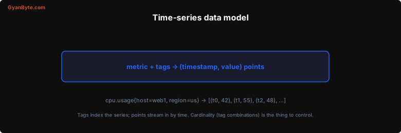
cpu.usage{host="web1", region="us-east"}  →  [(t0, 42), (t1, 55), (t2, 48), …]
http.latency_ms{route="/checkout", pod="p7"} →  [(t0, 120), (t1, 98), …]
The combination of metric name and tag values defines a series — one logical stream of points. Tags are what you filter and group by at query time (“average latency by route”). This model is both the power and the trap of time-series systems, which brings us to the one number you must mention.
Cardinality is the thing to control
Cardinality is the number of distinct series — every unique combination of metric name and tag values. cpu.usage with 10,000 hosts and 5 regions is up to 50,000 series. That is fine. The danger is putting a high-cardinality value in a tag: tagging by user_id, request_id, or a raw URL with unbounded path parameters can create millions or billions of series, each of which the database must track and index in memory. This is the single most common way to melt a time-series database.
The rule to state in an interview: tags should be low-cardinality dimensions you group by (host, region, route, status code), never unbounded identifiers. If you need per-request detail, that belongs in logs or traces, not metrics.
How the storage engine is built
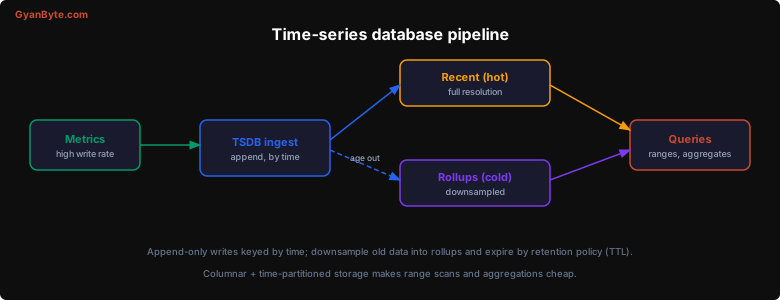
A time-series database makes a handful of design choices that directly match the four properties above:
- Append-only, LSM-style writes. New points are written sequentially (often buffered in memory, then flushed as immutable files), never updated in place — perfectly matched to the ingest pattern and the opposite of a B-tree’s random updates.
- Time-partitioned, columnar storage. Data is chunked into time blocks (e.g. per two hours or per day) and stored column-by-column. A range query reads only the blocks that overlap the time range, and an aggregate reads only the value column — so “average over the last hour” touches a tiny, contiguous slice of disk.
- Aggressive compression. Consecutive timestamps are near-regular and consecutive values change slowly, so delta-of-delta encoding for timestamps and XOR encoding for values (the Gorilla/Facebook technique) compress points to a couple of bits each. This is what lets a TSDB hold billions of points cheaply.
- Downsampling into rollups. A background job rolls recent high-resolution data into coarser summaries — raw points for the last few hours, 1-minute averages for the last week, 1-hour averages for the last year. Old queries read small rollups instead of huge raw ranges.
- Retention and TTL. Because value decays with age, the database drops whole old time-partitions on a schedule. Deletion is cheap — drop a file, not a billion rows.
Retention policy (illustrative):
  raw (10s)      → keep 48 hours
  1-min rollup   → keep 30 days
  1-hour rollup  → keep 2 years
The ecosystem and where it fits
The common systems split into a few shapes worth knowing:
| System | Shape | Reach for it when |
|---|---|---|
| Prometheus | Pull-based, local storage, alerting built in | Infrastructure/service monitoring in one cluster |
| InfluxDB | Push-based TSDB with its own query language | General metrics/IoT with flexible tags |
| TimescaleDB | Postgres extension (time-partitioned tables) | You want SQL and relational joins alongside time-series |
| Druid / ClickHouse | Columnar OLAP, also great at time-series | High-cardinality analytics and slice-and-dice dashboards |
Use cases are everywhere a value is tracked over time: metrics and monitoring (the canonical one — Prometheus scraping services, Grafana charting them), IoT and sensor telemetry, financial tick data, and application observability. When an interviewer asks you to “design a metrics / monitoring system,” the answer is an ingestion pipeline (often through Kafka to absorb bursts) feeding a time-series database, with downsampling and retention, a query layer for dashboards, and a rule engine for alerts — and the first thing you call out is controlling cardinality.
Key Takeaways
-
Time-series data is append-only, high-rate, and queried by range/aggregate. That shape — not any one feature — is why it needs a purpose-built database.
-
The model is metric + tags → (timestamp, value) points. Tags are the low-cardinality dimensions you group by.
-
Cardinality is the failure mode. Never tag by unbounded identifiers (user id, request id, raw URL); that explodes the number of series and the memory to track them.
-
The engine is append-only, time-partitioned, columnar, and heavily compressed. Range and aggregate queries touch only the relevant time blocks and the value column.
-
Downsample and expire. Roll old data into coarser rollups and drop whole old partitions by retention policy, because value decays with age.
-
It underpins metrics/monitoring designs. Prometheus, InfluxDB, TimescaleDB, or columnar stores like Druid/ClickHouse — pick by whether you need pull vs push, SQL, or high-cardinality analytics.