Stream Processing

Most of the designs so far store data and answer queries against it. Stream processing flips that around: instead of storing data and asking questions later, you ask the questions once and let a continuous flow of events answer them in real time. When an interviewer asks for “the number of clicks per ad in the last minute,” “trending hashtags right now,” or “alert me when error rates spike,” they are asking for a streaming system.

This lesson covers the pieces that show up in those designs and the vocabulary that signals you know how real-time data systems are built.

In the interview: the trigger phrases are “real-time,” “trending,” “live counts,” “aggregation over a firehose,” and “alert when…“. When you hear them, reach for a stream processor (Flink / Kafka Streams) fed by a durable log, and talk about windowing and late data — that is what separates a real answer from “I’ll just query the database.”

Batch vs stream

The distinction is about the shape of the data:

• Batch processing runs over a bounded dataset — a day’s worth of logs, a table, a file. The job starts, processes a finite input, produces output, and finishes. Think a nightly report or a MapReduce job. Latency is minutes to hours; throughput and completeness are the priorities.
• Stream processing runs over an unbounded dataset — an endless sequence of events that never “finishes.” The job runs forever, processing each event (or small window of events) as it arrives. Latency is milliseconds to seconds.

The reason streaming needs its own toolbox is precisely that the data never ends. You cannot “wait for all the data” before computing an average, because there is no end. Every hard concept below exists to answer the question: how do you compute aggregates over a stream that has no final boundary?

The pipeline

Almost every streaming system has the same four stages.

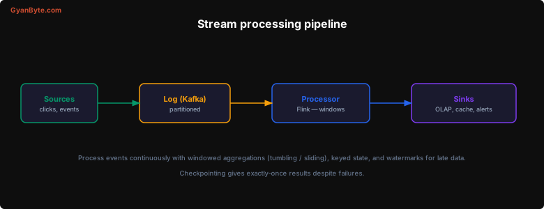
1. Sources — the producers of events: application servers emitting clicks, IoT sensors, database change logs, user activity. They emit a high-volume, continuous feed.
2. A durable log — almost always Kafka (or Kinesis / Pulsar). The log decouples producers from processors, buffers bursts, preserves ordering within a partition, and — critically — retains events so they can be replayed. The log is the backbone; everything downstream can be rebuilt from it.
3. A stream processor — Flink, Kafka Streams, or Spark Structured Streaming. This is where the actual computation lives: filtering, transforming, joining, and — the heart of it — windowed aggregation. The processor holds state and updates it as events flow through.
4. Sinks — where results land: an OLAP store (Druid, ClickHouse) for dashboards, a cache or key-value store for fast serving, an alerting system, or another Kafka topic for the next stage.

This structure composes with everything else in the course: the log is the Kafka you already know, and the sinks are the databases and caches from earlier lessons.

Windowing

You cannot average an infinite stream, so you chop it into windows — finite buckets of time (or count) over which an aggregate is computed. The three common kinds:

• Tumbling windows — fixed-size, non-overlapping buckets: “clicks per ad per 1-minute window.” Each event belongs to exactly one window. This is the workhorse for periodic counts.
• Sliding windows — fixed-size but overlapping, advancing by a smaller step: “average over the last 5 minutes, updated every 30 seconds.” An event belongs to multiple windows. Used for moving averages and rolling metrics.
• Session windows — dynamically sized, defined by gaps of inactivity: “group a user’s events until they are idle for 30 minutes.” The window length depends on the data. Used for user sessions and activity bursts.

Naming the window type and its size in a design (“I’ll keep tumbling 1-minute windows keyed by ad id”) is a concrete, credible answer.

Event time, processing time, and watermarks

Here is the subtlety that trips people up. There are two clocks:

• Processing time — when your processor sees the event.
• Event time — when the event actually happened at the source.

These differ because of network delays, retries, and devices that were offline and sync later. An event that happened at 12:00:59 might not reach your processor until 12:01:03 — after the 12:00–12:01 window has already “closed.” If you bucket by processing time, that click is miscounted into the wrong minute; aggregates computed during that window are wrong.

Correct streaming systems compute on event time, which raises the question: how long do you wait for stragglers before declaring a window complete? The answer is a watermark — a moving threshold that asserts “I believe I have now seen all events up to event-time T.” When the watermark passes the end of a window, the processor emits that window’s result and can drop late arrivals (or route them to a side output for correction). Watermarks are the mechanism that lets a system reason about completeness over data that arrives late and out of order.

State and exactly-once

A stream processor is stateful: to count clicks per ad, it must remember a running count per ad across events. This keyed state lives in the processor (backed by an embedded store like RocksDB, and periodically snapshotted).

The reliability question is what happens when the processor crashes mid-stream. Checkpointing is the answer: the processor periodically snapshots its state and its position (offset) in the input log, atomically. On recovery, it restores the last checkpoint and replays the log from the saved offset. Combined with idempotent or transactional sinks, this yields exactly-once processing — every event affects the result exactly once, even across failures. This is Flink’s headline guarantee and a strong thing to cite: “Flink gives me exactly-once via checkpointing, so a crash doesn’t double-count.”

Lambda vs Kappa architecture

How do you combine real-time results with historical accuracy? Two patterns:

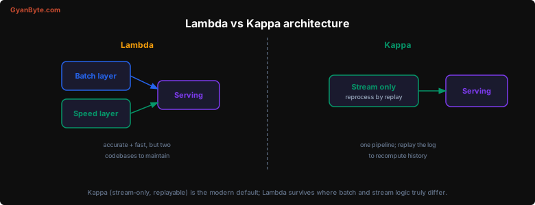
• Lambda architecture. Run two pipelines: a batch layer that recomputes accurate results over all historical data (slow, correct) and a speed layer that computes approximate real-time results (fast, recent). A serving layer merges them. The win is accuracy plus low latency; the pain is maintaining two codebases that must produce consistent results — the same aggregation logic implemented twice, in two systems, kept in sync forever.
• Kappa architecture. Run one streaming pipeline. Because the log (Kafka) retains history and can be replayed, you reprocess the past by simply replaying the log through the same stream job. No separate batch layer, no duplicated logic. To recompute, spin up a new version of the job reading from the beginning of the log.

Kappa has become the modern default: one pipeline, one codebase, with replay standing in for batch recomputation. Lambda survives mainly where the batch and streaming logic genuinely differ, or where a legacy batch system already exists. In an interview, propose Kappa and mention Lambda as the older alternative — it shows you know the evolution.

When to reach for it

Stream processing is the right tool when the design calls for:

• Real-time aggregation — counts, sums, averages over a high-volume feed (ad clicks, page views, metrics).
• Trending / top-K — what is popular right now, computed over a sliding window.
• Alerting and anomaly detection — react within seconds when a metric crosses a threshold.
• Continuous ETL — transform and route events as they arrive rather than in nightly batches.
• Stream joins / enrichment — join a live event stream against reference data.

If the question instead asks for occasional queries over stored data, a database or a batch job is simpler — do not reach for a streaming stack when a nightly job would do.

Key Takeaways

1. Batch is bounded, streaming is unbounded. Streaming’s entire toolbox exists to compute aggregates over data that never ends, with low latency.

2. The pipeline is sources → durable log → stream processor → sinks. Kafka decouples and retains (enabling replay); Flink / Kafka Streams does the stateful computation; results land in OLAP stores, caches, or alerts.

3. Window the stream. Tumbling (fixed, non-overlapping), sliding (overlapping, moving average), and session (gap-based) windows turn an infinite stream into finite, computable buckets.

4. Compute on event time with watermarks. Events arrive late and out of order; a watermark decides when a window is “complete enough” to emit, so results are correct despite stragglers.

5. Checkpointing gives exactly-once. The processor snapshots keyed state plus its log offset; on failure it restores and replays, so a crash does not double-count.

6. Prefer Kappa over Lambda. One replayable stream pipeline beats maintaining separate batch and speed layers with duplicated logic — reprocess history by replaying the log.