Databases Deep-Dive: Indexing and Transactions — Cracking the System Design Interview

Most candidates can say “I’ll use PostgreSQL” or “I’ll use Cassandra,” but freeze when the interviewer asks why — or what happens to writes when you add that index, or what isolation level you need. This lesson takes you one level below the component toolbox and into how databases actually store and protect your data. It is the difference between naming a database and reasoning about one.

By the end you’ll be able to justify an index, pick an isolation level, and choose SQL vs NoSQL from first principles rather than habit.

How a database finds a row: indexes

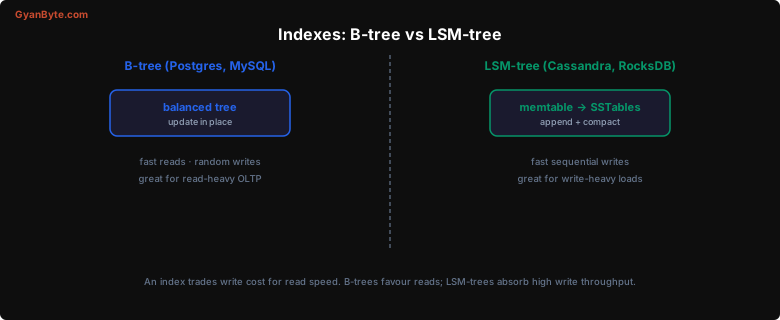
Without an index, finding a row means scanning the whole table — O(n). An index is a secondary data structure that turns that scan into a lookup. The two dominant index designs make opposite trade-offs, and knowing which engine uses which tells you what a database is good at.

B-tree vs LSM-tree indexes — B-trees update in place and favour reads, LSM-trees append to a memtable and compact into SSTables, favouring writes

B-tree: read-optimized, update-in-place

A B-tree keeps keys sorted in a shallow, balanced tree. A lookup walks from the root to a leaf in O(log n) — typically three or four disk pages even for billions of rows. This is the default index in PostgreSQL, MySQL (InnoDB), and most relational databases.

Reads are excellent: point lookups and range scans (WHERE age BETWEEN 20 AND 30) both ride the sorted structure.
Writes update the tree in place. A single row insert may have to split a page and update several nodes, causing random disk I/O.

B-trees shine on read-heavy and mixed OLTP workloads where you query many ways and need fast range scans.

LSM-tree: write-optimized, append-and-compact

A Log-Structured Merge-tree never updates in place. Writes go to an in-memory memtable; when it fills, it is flushed to disk as an immutable sorted file (an SSTable). A background compaction process merges SSTables and discards overwritten values. This design powers Cassandra, RocksDB, ScyllaDB, and many time-series stores.

Writes are sequential appends — extremely fast, which is why LSM engines absorb enormous write throughput.
Reads may have to check the memtable plus several SSTables, so they use Bloom filters to skip files that can’t contain the key.

LSM-trees win when writes dominate: event ingestion, metrics, messaging, feeds.

B-tree write:   find leaf → maybe split page → random I/O  (read-friendly)
LSM-tree write: append to memtable → flush → compact later (write-friendly)

What an index costs

An index is not free. Every write must update every index on the table — this is write amplification. A table with five indexes does roughly five times the write work of an unindexed one, plus the storage.

So the rule is: add indexes to match real query patterns, not speculatively.

Index the columns you filter and join on, not every column.
For a composite index (a, b, c), order the columns by selectivity and by how you query: it serves WHERE a = ?, WHERE a = ? AND b = ?, but not WHERE b = ? alone (the leftmost-prefix rule).
A covering index that includes every column a query needs lets the database answer from the index alone, skipping the table entirely.

Interview tip: When you draw a database, name the primary access pattern and the one or two indexes that serve it. “We query posts by user_id ordered by created_at, so I’ll put a composite index on (user_id, created_at)” shows you think about reads and the write cost they add.

Keeping data correct: transactions

A transaction groups several operations so they succeed or fail as a unit. The guarantees are summarised as ACID.

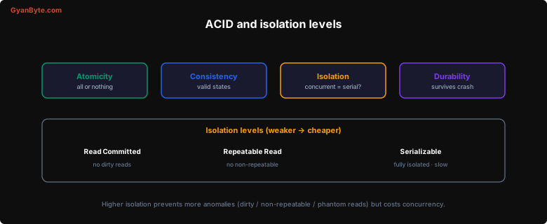
ACID properties — atomicity, consistency, isolation, durability — and isolation levels from read-committed to serializable with the anomalies each prevents

Atomicity — all operations commit, or none do. A transfer that debits one account must credit the other, or roll back entirely.
Consistency — every committed transaction leaves the database in a valid state (constraints, foreign keys hold).
Isolation — concurrent transactions behave as if they ran one at a time (to a degree you choose — see below).
Durability — once committed, the data survives a crash, usually via a write-ahead log flushed to disk.

Isolation levels: safety vs concurrency

Full isolation (every transaction appears to run alone) is expensive, so databases offer weaker levels that allow more concurrency by permitting specific anomalies. From weakest to strongest:

Level	Prevents	Still allows
Read Uncommitted	nothing	dirty reads
Read Committed	dirty reads	non-repeatable reads, phantoms
Repeatable Read	dirty + non-repeatable reads	phantom reads
Serializable	all of the above	(nothing — fully isolated)

The anomalies, in plain terms:

Dirty read — you read another transaction’s uncommitted change that may be rolled back.
Non-repeatable read — you read a row twice in one transaction and get different values because someone committed a change in between.
Phantom read — you run the same range query twice and new rows appear because someone inserted into that range.

Higher isolation prevents more anomalies but reduces concurrency and can cause more lock contention or serialization failures (which you must retry). Read Committed is the common default; reach for Serializable only where correctness truly demands it, such as financial ledgers.

MVCC in one line

Most modern databases use Multi-Version Concurrency Control: writers create new versions of rows instead of overwriting, so readers never block writers and writers never block readers — each transaction sees a consistent snapshot. It is why Postgres can run a long analytical read without freezing writes.

SQL vs NoSQL, one level deeper

The component lesson gave you the headline rule. Now the nuance.

Choose a relational (SQL) database when:

You need multi-row transactions and strong consistency (payments, inventory, bookings).
Your data is relational and you query it many ways with joins and aggregations.
The schema is stable and you benefit from constraints catching bad data.
Modern Postgres scales further than people assume — read replicas, partitioning, and JSONB cover a huge range before you ever need NoSQL.

Choose a NoSQL database when:

You need horizontal write scale beyond one primary (a wide-column store like Cassandra, or a managed key-value store like DynamoDB).
Your access pattern is simple and known: lookups by a partition key, not arbitrary ad-hoc queries.
The schema is flexible or varies per record (document stores like MongoDB).

The critical NoSQL decision is the partition key. In a system like DynamoDB or Cassandra you model the table around the query — the partition key determines which node holds the data, so it must spread load evenly and match how you read. A poorly chosen partition key (for example, a key that is “today’s date”) funnels all traffic to one hot partition and the system falls over, no matter how many nodes you have.

Interview tip: State your needs before you name a database. “This needs transactional correctness and relational queries, so PostgreSQL” or “this is write-heavy, keyed by device_id, and never joined, so Cassandra” is a complete, senior answer. Naming the database first and reasoning backwards is the junior tell.

Key Takeaways

An index trades write cost for read speed. B-trees favour reads and range scans; LSM-trees absorb heavy writes. Match the engine to the workload.
Every index amplifies writes. Add indexes to serve real queries, order composite-index columns by how you filter, and consider covering indexes for hot reads.
ACID is the contract; isolation level is the dial. Read Committed by default, Serializable only where correctness demands it — and remember stronger isolation costs concurrency.
MVCC lets readers and writers proceed without blocking each other by keeping multiple row versions.
Pick the store from the requirement. Transactions, joins, stable schema → SQL. Horizontal write scale, simple key-based access, flexible schema → NoSQL, and the partition key is the decision that makes or breaks it.