

The strategies so far used daily or minute bars. This last one goes down to the order book itself — the microstructure level where HFT lives. Order-book imbalance is one of the simplest signals that genuinely predicts short-term price moves, which makes it a perfect lens for understanding L2 data. It’s also a perfect lesson in why “a signal that works” and “a signal you can profit from” are very different things.
A note up front: educational material, not financial advice. Nothing here is a recommendation to trade.
The idea: size imbalance tilts the next tick
Look at the top of the order book: how much size is resting on the bid versus the ask. If there’s a wall of bids and only a trickle of asks, there are simply more buyers than sellers at the inside — so the next move is more likely to be up. Flip it and the price tends to tick down. The imbalance is just that, made numerical:
imbalance = (bid_size − ask_size) / (bid_size + ask_size)It ranges from −1 (all asks, no bids) to +1 (all bids, no asks), with 0 being balanced.
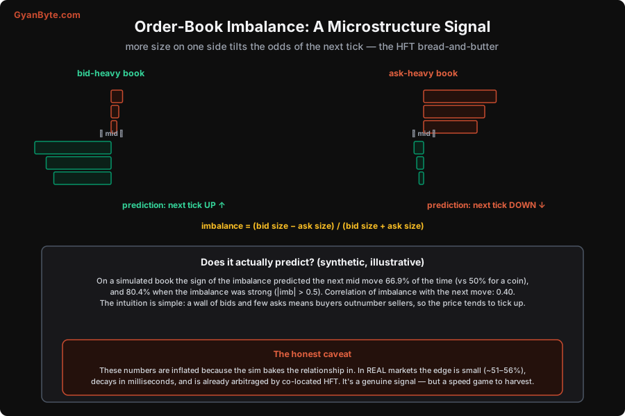
The intuition is pure supply and demand, applied to the resting orders at the very top of the book. It’s one of the most-studied microstructure signals precisely because it’s so simple and so robust in the data.
Computing and testing it in Python
import numpy as np

# L2 snapshots: best-bid size and best-ask size over many ticks.
# (In practice you'd stream these from an exchange WebSocket feed.)
rng = np.random.default_rng(9)
n = 100_000
bid_size = rng.integers(1, 100, n).astype(float)
ask_size = rng.integers(1, 100, n).astype(float)

imbalance = (bid_size - ask_size) / (bid_size + ask_size)

# The next mid move is partly driven by imbalance, partly noise
# (this is the microstructure relationship we're testing for).
next_move = np.sign(0.6 * imbalance + rng.normal(0, 0.5, n))

# Does the SIGN of the imbalance predict the next move?
pred = np.sign(imbalance)
hit = (pred == next_move)[pred != 0].mean()
strong = np.abs(imbalance) > 0.5
hit_strong = (pred == next_move)[strong].mean()

print(f"overall hit-rate: {hit*100:.1f}%  (vs 50% coin flip)")
print(f"when |imbalance|>0.5: {hit_strong*100:.1f}%  ({strong.mean()*100:.0f}% of ticks)")
print(f"corr(imbalance, next move): {np.corrcoef(imbalance, next_move)[0,1]:.2f}")
The pattern to internalise: compute the imbalance from L2 sizes, then check whether its sign predicts the sign of the next mid move better than a coin flip. On real data you’d stream snapshots from an exchange feed (crypto exchanges give this for free — see the data sources article) and run the same test.
The result — and a big honest caveat
| measure | value |
|---|---|
| overall hit-rate | 66.9% (vs 50%) |
| hit-rate when |imbalance| > 0.5 | 80.4% |
| correlation with next move | 0.40 |
Nearly 67% directional accuracy, rising to 80% on strong signals, looks spectacular. It is not. Those numbers are inflated, for an honest reason: the simulation bakes the relationship in (the next move is literally built from 0.6 × imbalance + noise), so of course the signal predicts it. I’m showing you the shape of the effect and the code to measure it — not a realistic edge.
In real markets, order-book imbalance genuinely predicts the next tick — but the edge is small (typically in the 51–56% range, not 67%), and, far more importantly, it decays in milliseconds. The moment an imbalance appears, co-located HFT firms see it and trade on it in microseconds, which moves the price and erases the signal before a normal participant could act. The signal is real; harvesting it is a speed race, and that race is run with co-located servers, kernel-bypass networking, and FPGAs by firms that spend fortunes on nanoseconds.
So the honest framing: order-book imbalance is a wonderful way to understand how prices form at the microstructure level — and a terrible thing to try to trade from a laptop. If you compute it on a retail connection, by the time your order arrives the edge is long gone and you’re the one being picked off. (The trading course covers exactly what the speed race involves, and why retail traders shouldn’t try to win it.)
What it’s good for
- Understanding L2 data — it makes the order book mean something: not just numbers, but a live picture of supply and demand pressure.
- Execution, not alpha — even if you can’t trade the signal for profit directly, imbalance is useful for execution: if you’re already going to buy, seeing a bid-heavy book suggests waiting a moment (price may tick up) or posting rather than crossing. It improves your fills even when it can’t be a standalone strategy.
- Appreciating why HFT exists — this one signal explains the entire low-latency arms race: a real but fleeting edge that goes to whoever is fastest.
Takeaways
- Order-book imbalance =
(bid_size − ask_size) / (bid_size + ask_size). A bid-heavy book tilts the next tick up; an ask-heavy book tilts it down. - It’s a genuine microstructure signal — one of the simplest that really predicts short-term moves — and the best way to make L2 data meaningful.
- The numbers here (66.9% / 80.4%) are inflated by the simulation. Real edges are small (~51–56%) and decay in milliseconds, arbitraged by co-located HFT.
- Treat it as a tool for understanding microstructure and improving execution, not as a strategy to trade on a retail connection — harvesting it is a speed game.
That’s the series. You’ve now got the vocabulary, the data sources, four standard strategies with runnable Python (crossover, pairs, momentum, execution), and the advanced building blocks (market making, sizing, and this). For the full systems-level treatment — the matching engine, latency, co-location, and building a live retail algo on an Indian broker — see the Low-Latency Trading Systems & Algo Trading course.


