

The moving-average crossover bet on direction and lost. Here’s a strategy with a genuinely different shape: it doesn’t care which way the market goes at all. Pairs trading is the entry point to statistical arbitrage, and it’s one of the most instructive ideas in quant trading because it makes “market-neutral” concrete.
A note up front: educational material, not financial advice. Nothing here is a recommendation to trade.
The idea: trade the spread
Take two assets that tend to move together — two banks in the same sector, a stock and its sector ETF, gold and a gold-miner. Most of the time they rise and fall in tandem, because the same forces drive both. Occasionally one gets ahead of the other and they drift apart — and historically, they tend to snap back.
So instead of betting on either asset’s direction, you bet on the spread between them reverting to its normal relationship:
- Form the spread:
spread = B − β·A, where β (the hedge ratio) is how many units of A move with one unit of B. - Measure how stretched it is with a z-score (how many standard deviations from its recent mean).
- When the spread stretches to +2σ, it’s unusually wide → short the spread (short B, long A), betting it narrows.
- At −2σ → long the spread (long B, short A).
- Exit near 0 (the mean).
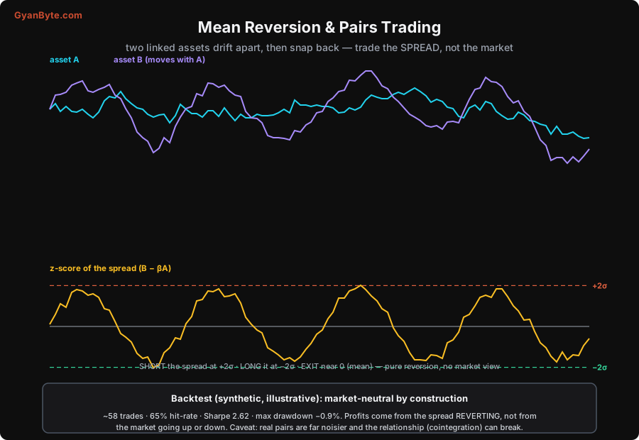
Because you’re long one asset and short the other in balanced amounts, a market-wide move up or down roughly cancels out. Your P&L comes almost entirely from the spread reverting, not from market direction. That’s what “market-neutral” means, and it’s the whole appeal.
The backtest, in full
import numpy as np
import pandas as pd
import yfinance as yf

# 1. Two assets that move together (e.g. two large-cap banks)
data = yf.download(["HDFCBANK.NS", "ICICIBANK.NS"], start="2019-01-01",
                   auto_adjust=True)["Close"].dropna()
A, B = data["HDFCBANK.NS"], data["ICICIBANK.NS"]

# 2. Hedge ratio (how much B moves per unit of A), via least squares
beta = np.polyfit(A, B, 1)[0]
spread = B - beta * A

# 3. Rolling z-score of the spread (60-day window)
z = (spread - spread.rolling(60).mean()) / spread.rolling(60).std()

# 4. Position logic: enter at ±2σ, exit inside ±0.5σ
pos = pd.Series(0.0, index=z.index)
for i in range(1, len(z)):
    prev = pos.iloc[i-1]
    if prev == 0:
        if z.iloc[i] > 2:    pos.iloc[i] = -1    # short the spread
        elif z.iloc[i] < -2: pos.iloc[i] = 1     # long the spread
    elif abs(z.iloc[i]) < 0.5:
        pos.iloc[i] = 0                           # exit near the mean
    else:
        pos.iloc[i] = prev                        # hold
pos = pos.shift(1).fillna(0)                      # act on yesterday's signal

# 5. P&L of the spread position (dollar-neutral), and a Sharpe
pnl = pos * spread.diff().fillna(0)
daily = pnl / (A.mean() + beta * B.mean())        # return on deployed capital
sharpe = daily.mean() / daily.std() * np.sqrt(252)
hit = (pnl[pos != 0] > 0).mean()
print(f"Sharpe {sharpe:.2f}   hit-rate {hit*100:.0f}%   trades {int(pos.diff().abs().sum()/2)}")
The structure is the same loop as before — build a signal, lag it, compute P&L — but the signal is the z-score of a spread rather than a price crossover, and the position holds two assets at once.
The result — and why to distrust it
On a synthetic pair that reverts cleanly, this looks superb:
| metric | value |
|---|---|
| Sharpe | 2.62 |
| hit-rate | 65% |
| max drawdown | −0.9% |
| trades | ~58 |
A Sharpe of 2.6 with a tiny drawdown is the kind of number that makes people quit their jobs. Don’t. That result is flattering, for a specific reason: synthetic data reverts by construction, so the strategy’s core assumption is guaranteed true. Real markets are far noisier, the spread wanders longer and wider, and — the real killer — the relationship can break.
The real risk: cointegration decay
Pairs trading assumes the two assets are cointegrated: linked by a relationship that holds over time, so the spread is mean-reverting. The danger is that this relationship stops holding. One bank has a scandal; one company’s business model diverges from its peer’s; a sector splits. Now the spread you’re betting will “revert” just keeps widening — and because you’re short the winner and long the loser, a persistent divergence bleeds you continuously. Your stop-loss fires, or worse, you average in expecting reversion that never comes. This is how market-neutral strategies blow up: not from market moves, but from the pair quietly ceasing to be a pair.
So in practice, serious pairs trading adds: a statistical test for cointegration (and re-testing it, because it decays), a stop-loss for when the spread keeps diverging, a basket of many pairs so no single break is fatal, and careful attention to costs (you’re trading two legs, and shorting has borrow costs). The idea is elegant; making it survive contact with real markets is the hard part.
Takeaways
- Pairs trading is market-neutral: trade the spread between two co-moving assets, not their direction. Profit from the spread reverting to its mean.
- The recipe: hedge ratio → spread → rolling z-score → enter at ±2σ, exit near 0. Long one leg, short the other.
- A great backtest Sharpe is a warning sign, not a green light — synthetic (and over-fit) data reverts too cleanly.
- The real risk is cointegration breaking: the pair permanently diverges and the “reverting” spread never reverts. Test it, stop-loss it, diversify it.
Next: a strategy whose edge is defensive — momentum and trend following, which earns its keep by sidestepping crashes. For the broader strategy families and options selling, see the strategies lesson in the course.


