How LLM Inference Uses Your Hardware — Open LLMs in Production — Serving, Quantization, Fine-Tuning and Cost

When people first benchmark an LLM, they’re often confused by a result like this: the model processes a 500-word prompt almost instantly, then generates its 200-word answer slowly, one word at a time. Same model, same hardware, wildly different speeds. Is something broken?

No. Those are the two phases every LLM request goes through, and they stress completely different parts of your hardware. Understanding this one thing explains almost everything else in this course: why decode is slow, why quantization helps, why batching helps, why a bigger model is proportionally slower, and what hardware to buy. Let’s build the mental model and then measure it.

Two Phases: Prefill and Decode

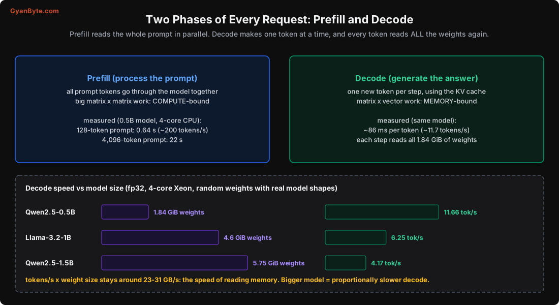
Two phases of every request. Prefill processes the whole prompt together in big matrix-matrix operations and is compute-bound; measured on a 0.5B model on a 4-core CPU, a 128-token prompt took 0.64 s (about 200 tokens/s) and a 4,096-token prompt took 22 s. Decode generates one new token per step using the KV cache, in matrix-vector operations that are memory-bound; measured on the same model, about 86 ms per token (11.7 tokens/s), with each step reading all 1.84 GiB of weights. Decode speed vs model size on CPU: Qwen2.5-0.5B 1.84 GiB at 11.66 tok/s, Llama-3.2-1B 4.60 GiB at 6.25 tok/s, Qwen2.5-1.5B 5.75 GiB at 4.17 tok/s; tokens/s times weight size stays around 23-31 GB/s, the speed of reading memory

Prefill (also called the “prompt” phase) happens first. The model reads your entire prompt at once. All the prompt’s tokens go through the network together, which means big matrix-by-matrix multiplications. Modern hardware is very good at these; they keep the compute units busy. So prefill is compute-bound: its speed is limited by how many floating-point operations per second your chip can do. It produces the first output token and, crucially, fills the KV cache (Lesson 3) with the prompt’s keys and values.

Decode (the “generation” phase) happens next. The model generates the answer one token at a time. To produce each new token, it runs a forward pass, but now the input is just the single previous token, so the multiplications are matrix-by-vector. These don’t keep the compute units busy. Instead, the bottleneck is reading all the model’s weights from memory to do that one small multiplication. Every single token requires reading the entire set of weights again. So decode is memory-bandwidth-bound: its speed is limited by how fast you can move the weights from memory into the compute units.

This asymmetry is the heart of LLM serving:

Prefill: lots of tokens, done together, limited by compute.
Decode: one token at a time, limited by memory bandwidth.

Measuring It on a Real Machine

I ran these on a plain 4-core Xeon VM with no GPU, using small models built from real architectures (Qwen2.5 and Llama shapes) with random weights. Random weights give meaningless text, but the timing is real: the same matrix multiplications and memory reads happen regardless of what the numbers are.

Prefill speed (time to process the prompt and produce the first token), on the 0.5B model:

prompt   128 tokens: prefill   0.64 s   (~200 tokens/s)
prompt 1,024 tokens: prefill   4.18 s   (~245 tokens/s)
prompt 4,096 tokens: prefill  22.1 s    (~185 tokens/s)

Prefill chews through roughly 200 tokens per second here. (It actually slows down a little at very long prompts because attention cost grows faster than linearly, more on that in Lesson 7.)

Decode speed, same 0.5B model: about 86 ms per token, or 11.7 tokens per second. That’s much slower per token than prefill, exactly as the model predicts.

These absolute numbers are CPU-slow; a GPU is 50-100x faster. But the shape of the result, prefill fast per token and compute-bound, decode slow per token and memory-bound, is identical on a GPU.

The Rule of Thumb for Decode Speed

Here’s the useful part. If decode is limited by reading all the weights once per token, then:

decode tokens per second (per user) ≈ memory bandwidth (GB/s) ÷ model size in memory (GB)

Let’s test it. I measured decode speed for three model sizes and computed tokens/s × model size:

Qwen2.5-0.5B  1.84 GiB  11.66 tok/s  ->  effective 23.0 GB/s
Llama-3.2-1B  4.60 GiB   6.25 tok/s  ->  effective 30.9 GB/s
Qwen2.5-1.5B  5.75 GiB   4.17 tok/s  ->  effective 25.7 GB/s

The “effective bandwidth” is roughly constant (23-31 GB/s) across very different model sizes. That’s the signature of a memory-bound process: the model reads its whole weight set per token, so speed is simply bandwidth divided by size. (For reference, a plain memory copy on this box measured about 45 GB/s; decode reaches a good fraction of that.)

Two immediate consequences:

A model twice the size decodes about half as fast. 70B is roughly 10x slower to decode than 7B, on the same hardware, before any other tricks.
The number that matters for decode speed is memory bandwidth, not teraflops. This is why an “AI PC” with lots of compute but ordinary RAM is slow at LLM decode, and why a Mac with fast unified memory is surprisingly good.

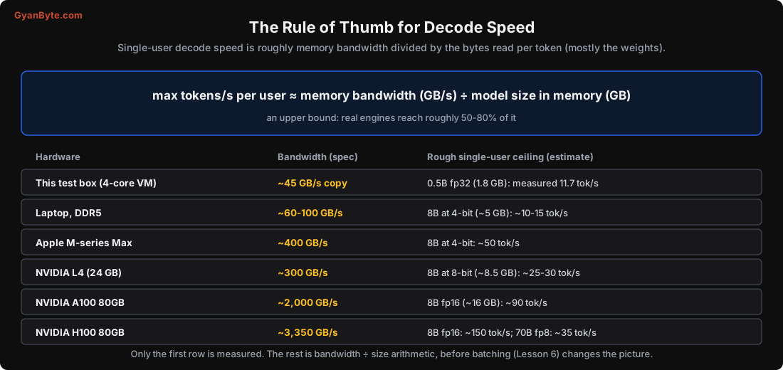
Only the first row of that table is measured on this machine. The rest is the bandwidth-÷-size estimate using each chip’s spec sheet. Real engines reach maybe 50-80% of the ceiling, and batching changes the picture completely (Lesson 6), but as a back-of-envelope sanity check, this rule is remarkably good. If a vendor claims a number far above bandwidth ÷ size for single-user decode, be skeptical.

Why This Shapes Every Later Decision

Keep this model in your head; the rest of the course is largely its consequences:

Quantization (Lesson 4): making the weights smaller (INT8, INT4) means fewer bytes to read per token, so decode gets faster and uses less memory. It barely helps compute-bound prefill, but it directly speeds up memory-bound decode.
Batching (Lesson 6): since decode reads the weights anyway, you can serve many users’ tokens in the same read, almost for free, on hardware with spare compute (a GPU). This is why one GPU serves dozens of users, and why per-user cost falls with utilisation.
KV cache (Lesson 3): the thing that makes decode need only the last token as input (instead of re-reading the whole prompt every step) is the KV cache. It trades memory for a huge amount of repeated compute.
Hardware choice: for throughput, you want memory bandwidth and enough memory to hold the weights plus KV cache. Compute matters most for prefill-heavy workloads (long prompts, RAG, classification of long documents).
Prompt length (Lesson 7): a long prompt means a long prefill (compute) before the first token appears. This is why time-to-first-token grows with prompt size.

Prefill-Heavy vs Decode-Heavy Workloads

One practical refinement: not all workloads have the same balance.

Chatbots and assistants: short-to-medium prompts, medium answers. A mix, with decode usually dominating the user’s wait.
RAG and long-context: huge prompts (retrieved documents, 3,000-10,000 tokens), short answers. Prefill-dominated; you’re paying mostly for compute on the input. Prefix caching (Lesson 7) attacks exactly this.
Classification and extraction: a document in, a short label or JSON out. Heavily prefill-dominated.
Long-form generation (write an article, generate code): short prompt, long output. Decode-dominated; memory bandwidth is king.

Knowing which one you have tells you what to optimise and what hardware to buy. There’s no point buying a compute monster for a decode-dominated workload, or chasing memory bandwidth for a classification service that’s all prefill.

Pitfalls to Avoid

Treating prefill and decode as one number. They have different bottlenecks; optimise them separately.
Buying for teraflops when your workload is decode-heavy. Memory bandwidth sets single-user decode speed.
Expecting quantization to speed up prefill much. It mainly helps memory-bound decode (and fit).
Benchmarking with one user and quoting that as capacity. Batching changes throughput by a large factor (Lesson 6).
Ignoring prompt length in latency. A long prompt is a long prefill before any token appears.
Assuming a bigger model is “a bit” slower. Decode time scales roughly with model size: 10x bigger is about 10x slower per token.

Quick Recap

Every request has two phases: prefill (whole prompt, compute-bound, fast per token) and decode (one token at a time, memory-bound, slow per token).
Measured: prefill ~200 tokens/s, decode ~11.7 tokens/s (86 ms/token) for a 0.5B model on CPU.
Decode is memory-bandwidth-bound: tokens/s × model size stayed around 23-31 GB/s across model sizes, so a model twice the size decodes about half as fast.
Rule of thumb: decode tokens/s ≈ memory bandwidth ÷ model size in memory.
This is why quantization, batching and fast memory matter, and why your workload’s prefill/decode balance decides what to optimise.

Next lesson: the actual memory maths. Exactly how much memory the weights take at each precision, and the KV cache that grows with every token and decides how many users you can serve at once.