ETL vs ELT & Modelling — Data Engineering: Building Data Pipelines — From Raw Events to a Trustworthy Warehouse

Data has landed (Lesson 3) and is stored well (Lessons 4–6). Now it must become useful — cleaned, joined, aggregated, and shaped into tables that answer business questions. That is transformation, and two things about it are worth a lesson: where the transform happens (the shift from ETL to ELT), and what shape you transform toward (dimensional modelling).

ETL Became ELT

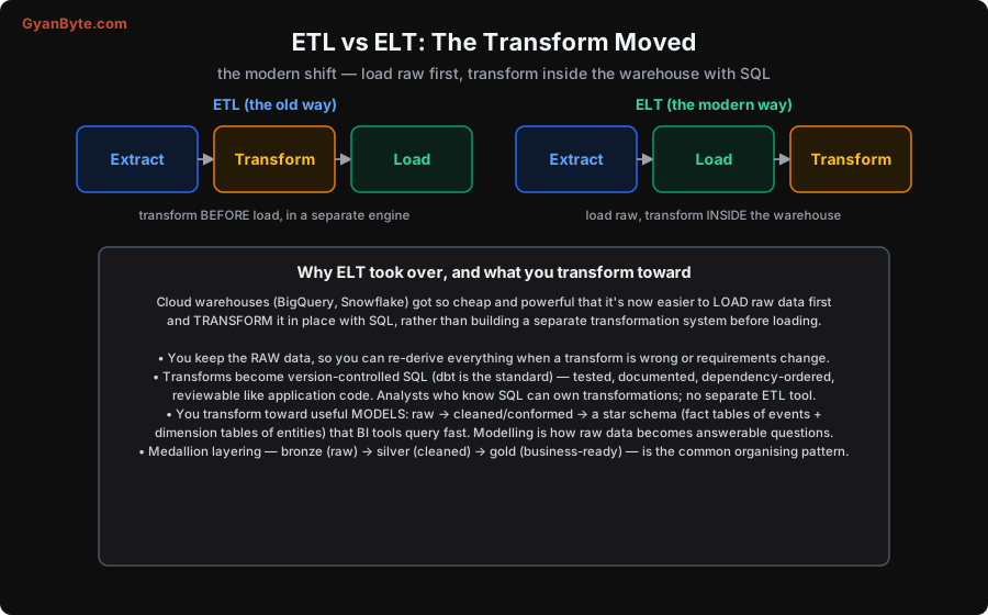
The classic approach was ETL — Extract from the source, Transform the data in a separate processing system, then Load the clean result into the warehouse. Transformation happened before loading, in its own engine, because warehouses used to be expensive and relatively weak, so you did the heavy lifting elsewhere and only loaded the polished result.

The modern approach is ELT — Extract, Load the raw data into the warehouse first, then Transform it in place with SQL. The order of the last two letters swapped, and it changed everything. Why? Cloud warehouses (BigQuery, Snowflake, Redshift) and query engines got so cheap and powerful that it’s now easier and faster to load raw data straight in and transform it where it already sits, using the warehouse’s own massive compute, than to build and run a separate transformation system upstream.

ELT isn’t just a reordering; it brings real advantages:

You keep the raw data. Because you load before transforming, the original untouched data is right there in the warehouse. When a transform has a bug, or the business changes what it wants, you re-run the transform on the raw data — you never lost it. (This is the “land raw first” principle from Lesson 3, realised.) ETL, which transformed before loading, often threw the raw away.
Transforms become code. The transformation is now just SQL running in the warehouse — and the tool that organises it, dbt (data build tool), has become the industry standard. dbt turns your transforms into version-controlled, tested, documented, dependency-ordered SQL models: each model is a SELECT that builds a table from other models, dbt works out the dependency graph and runs them in order, and you write tests (uniqueness, not-null, referential integrity — Lesson 11) alongside. Transformations become reviewable, testable code like any application — and because it’s just SQL, analysts who know SQL can own them, no separate ETL engineering tool required.

So the modern transform layer is: load raw, then build a graph of tested SQL models (dbt) inside the warehouse that refine raw data into business-ready tables.

What You Transform Toward: Dimensional Modelling

Transforming isn’t just cleaning — it’s shaping data into a model that makes analytical questions easy and fast to answer. The dominant design, from Ralph Kimball, is dimensional modelling, and its central structure is the star schema.

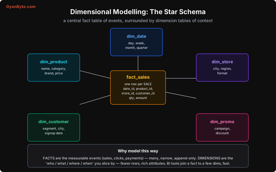
The star schema splits your data into two kinds of table:

A fact table holds the measurable events — one row per sale, click, payment, order line. Fact tables are many rows, narrow (a few measures like qty and amount, plus foreign keys to dimensions), and append-only. fact_sales with a row per sale is the classic example.
Dimension tables hold the context you slice by — the “who, what, where, when.” dim_product (name, category, brand), dim_store (city, region), dim_customer (segment), dim_date (day, week, month, quarter). Dimensions are fewer rows, rich with descriptive attributes.

A fact table surrounded by its dimensions looks like a star, hence the name. Analytical queries then join a fact to a few dimensions and aggregate: “sum amount from fact_sales, joined to dim_date and dim_store, grouped by month and region.” This shape is deliberately optimised for how analysts and BI tools query — it’s intuitive (“I want sales by product by month”), it keeps the huge fact table lean (context lives in the small dimensions, not repeated on every fact row), and warehouses execute star-schema joins very efficiently. Modelling your raw data into clean facts and dimensions is how you turn “we have the data somewhere” into “analysts can answer questions in seconds.”

Organising the Transform: Medallion Layering

One more pattern ties it together: you don’t go from raw to star schema in one giant leap. The common organising convention is medallion layering (bronze → silver → gold):

Bronze — raw, as-ingested data (Lesson 3’s landing zone). Untouched, the source of truth you can always re-derive from.
Silver — cleaned and conformed: deduplicated (Lesson 11), types fixed, columns standardised, joined into sensible entities. The “trustworthy, cleaned” layer.
Gold — business-ready: the star-schema facts and dimensions, aggregates, and metrics that BI tools and analysts actually query.

Each layer is built from the one below with tested SQL models (dbt), so the pipeline is a clear, debuggable progression from raw mess to modelled answers. When a number looks wrong, you trace it back down the layers to find where it went astray. This layered, tested, version-controlled approach is what makes transformation maintainable rather than a pile of opaque scripts — and it’s the backbone of a modern analytics stack. Next we look under the hood at the engines that execute these transforms at scale.

Pitfalls to Avoid

Transforming before loading and discarding the raw. Old-style ETL that throws away the source means a transform bug loses data you can’t recover. Load raw first (ELT/bronze), keep it, and re-derive — always.
Transformations as opaque, untested scripts. A pile of ad-hoc SQL/Python with no tests, no dependency order, no version control rots fast. Use dbt (or equivalent): version-controlled, tested, dependency-ordered models.
No data modelling — querying raw tables directly. Pointing BI tools at raw, un-modelled tables gives slow, confusing queries and duplicated logic. Model into a star schema (facts + dimensions) so queries are fast and intuitive.
Fat fact tables with context baked in. Repeating product name, category, region on every fact row bloats the biggest table and makes changes painful. Put descriptive attributes in dimensions; keep facts narrow (keys + measures).
Skipping the cleaned (silver) layer. Jumping from raw straight to business metrics bakes dirty data into the gold layer. Clean and conform first (dedup, types, standardisation), then model.
Assuming ELT means “no transformation discipline.” Loading raw is easy; the discipline is in the tested model graph that refines it. ELT without dbt-style rigour just moves the mess into the warehouse.

Quick Recap

The transform moved: ETL (transform before load, in a separate engine) became ELT (load raw, transform in-warehouse with SQL) because cloud warehouses got cheap and powerful.
ELT’s wins: you keep the raw data (re-derive when transforms change or break), and transforms become version-controlled, tested, dependency-ordered SQL — dbt is the standard, and SQL-literate analysts can own it.
You transform toward a model: the star schema — a central fact table (events: many, narrow, append-only) surrounded by dimension tables (context: who/what/where/when, rich attributes). BI queries join a fact to a few dims and aggregate — intuitive and fast.
Organise the pipeline as medallion layers: bronze (raw) → silver (cleaned/conformed) → gold (star schema, business-ready), each built from the last with tested models.

Next lesson: the engines that execute these transforms at scale — distributed processing and why the shuffle is the expensive part (with a measured single-node baseline).