Distributed Processing — Data Engineering: Building Data Pipelines — From Raw Events to a Trustworthy Warehouse

Some transforms (Lesson 7) run over data far too big for one machine’s memory — billions of rows, terabytes of files. Distributed processing engines like Apache Spark handle this by spreading the work across a cluster. Understanding how they do it — and specifically why one step, the shuffle, dominates the cost — is what separates engineers who can make big jobs fast from those who just throw more machines at them. This lesson is that mental model, with a measured reminder not to over-reach for a cluster.

Map, Shuffle, Reduce

Distributed processing and the shuffle: how engines split work across machines and why the shuffle is the expensive part. Data is split into partitions (part 0, part 1, part 2, part 3). Then a SHUFFLE — rows re-partitioned by key across the network (the costly step) — regroups them into groups (grp 0..3) grouped by key, then aggregate. What to know (and a measured baseline): engines like Spark split data into partitions, process them in parallel (MAP), then must SHUFFLE — move rows across the network so all rows with the same key land together — before a GROUP BY or JOIN (REDUCE); the shuffle is network plus disk heavy and is where most jobs spend their time; SKEW (Lesson 6) makes one reducer the bottleneck; minimise and balance shuffles: filter early, pick good keys, avoid needless re-partitioning; you don't always need a cluster: measured, DuckDB aggregated 2,000,000 rows in 64 ms (about 31M rows/sec) on ONE machine, about 22 times faster than a naive Python loop; reach for Spark at genuinely big scale, single-node engines go far.

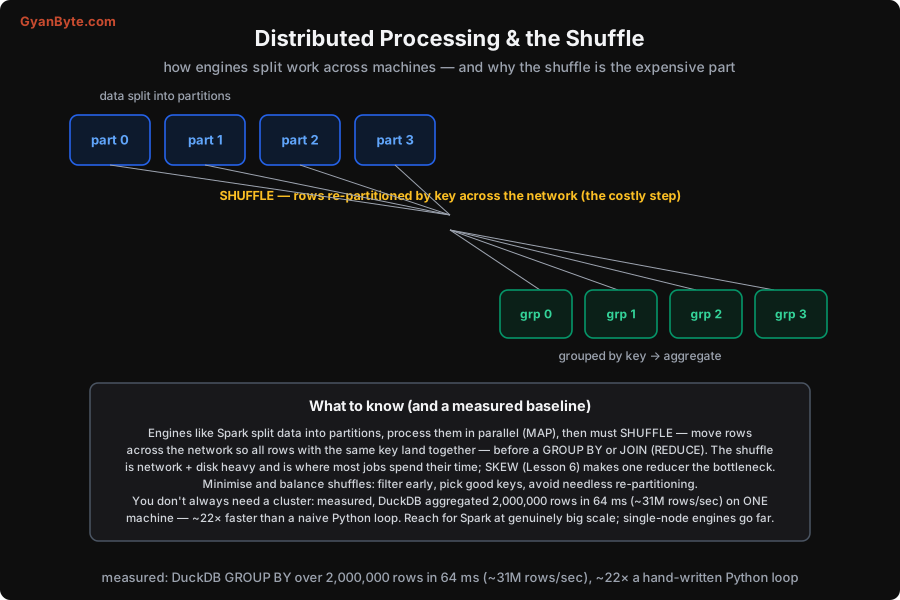
The core model (it’s the old MapReduce idea, and Spark’s too) has three phases:

Partition + Map. The data is split into partitions (chunks), spread across the cluster’s machines, and each machine processes its partitions in parallel — filtering, projecting columns, computing per-row values. This phase scales beautifully: more machines, more partitions processed at once, no coordination needed. This is the easy, cheap part.
Shuffle. Here’s the catch. To do a GROUP BY or a JOIN, all the rows with the same key must end up on the same machine — but after the map phase, rows with a given key are scattered across every partition on every machine. So the engine must shuffle: re-partition the data by key, physically moving rows across the network (and spilling to disk) so that, say, all the city = Mumbai rows land together. The shuffle is an all-to-all data movement, and it is by far the most expensive part of most jobs — network and disk I/O dwarf the CPU of the map phase.
Reduce. Now that each key’s rows are co-located, each machine computes the final result for its keys — summing, counting, joining. Cheap again, like the map phase.

The whole art of making distributed jobs fast is managing the shuffle, because that’s where the time goes.

Why the Shuffle (and Skew) Dominate

Three things follow from “the shuffle is the expensive part”:

Minimise how much you shuffle. Filter and aggregate early — before the shuffle — so fewer rows and columns cross the network. This is where columnar storage pays off again: predicate pushdown and column projection (Lesson 4) let the engine read only the needed columns and skip non-matching row groups at the source, so the data entering the shuffle is as small as possible. Reducing bytes shuffled is usually the single biggest speed-up available.
Avoid needless shuffles. Each GROUP BY/JOIN/re-partition can trigger a shuffle. Structuring a job to shuffle once instead of three times, or using a broadcast join (ship a small table to every machine instead of shuffling the big one), can transform its runtime. Experienced engineers read a query plan specifically to count and shrink the shuffles.
Beware skew — it makes one reducer the bottleneck. This is Lesson 6’s skew, now with teeth. After the shuffle, if one key holds most of the rows (the hot key that was 70% of data, making one partition 5.9× the average), then one reducer gets most of the work while the others finish and idle. And because a distributed job’s wall-clock is set by its slowest task, that one overloaded reducer determines the whole job’s runtime. Skew in a shuffle key is the classic “why is this job taking forever when I added more machines?” culprit — the extra machines sit idle waiting for the straggler. Fix it by salting the hot key or handling it separately (Lesson 6).

Get those right — small shuffles, few shuffles, no skew — and a distributed job flies. Ignore them and no amount of extra cluster capacity will save you, because you’re bottlenecked on network movement and a single straggler, not on raw compute.

You Don’t Always Need a Cluster (measured)

A crucial, money-saving caveat: distributed processing has real overhead — a cluster to provision and operate, the shuffle’s network cost, coordination — and it only pays off when the data genuinely doesn’t fit on one machine. Teams routinely reach for Spark on data that a single modern machine would chew through in seconds.

I measured a reminder of this. Aggregating 2,000,000 rows (GROUP BY city, SUM(amount)) with DuckDB — a single-node, in-process, columnar, vectorised engine — took 64 ms (~31 million rows/sec) on one machine, and that was ~22× faster than a naive Python loop doing the same thing. A single-node engine using columnar formats and vectorised execution handles a surprising amount of data — tens or hundreds of millions of rows, often into the billions — with no cluster at all. DuckDB and Polars have made “just run it on one big machine” viable for a huge fraction of workloads that reflexively used to go to Spark.

So the practical stance: reach for Spark (or a distributed warehouse) at genuinely big scale — when the data truly exceeds one machine, or you need the cluster’s parallelism. For everything below that, a single-node engine is simpler, cheaper, and often faster (no shuffle across a network, no cluster startup). A cluster you don’t need is cost and complexity you don’t need. Measure your actual data size before assuming you need to distribute — the honest answer is often “this fits on one box.” And when you do distribute, remember the lesson: the shuffle and skew, not the row count, decide how fast the job runs.

Pitfalls to Avoid

Ignoring the shuffle. Treating a distributed job as “just add machines” misses that the shuffle (network/disk movement for group-by/join) is where the time goes. Minimise bytes shuffled (filter/aggregate early) and the number of shuffles.
Skew in the shuffle key. One hot key overloads one reducer, and wall-clock follows the slowest task — so more machines don’t help. Detect skew and salt/split the hot key (Lesson 6).
Not filtering/projecting before the shuffle. Shuffling columns and rows you’ll later discard wastes the expensive step. Use predicate pushdown and column projection (columnar, Lesson 4) to shrink data before it moves.
Reaching for Spark on small data. A cluster’s overhead (provisioning, coordination, shuffle) isn’t worth it for data a single machine handles — measured, DuckDB did 31M rows/sec on one box. Check your real data size first.
Shuffling a big table to join a small one. Joining a huge fact to a tiny dimension by shuffling both is wasteful; broadcast the small table to every worker instead. Know your engine’s broadcast/hash-join options.
Adding machines to fix a skewed or shuffle-bound job. If the bottleneck is one straggler or network movement, more workers sit idle. Fix the shuffle/skew; scaling out only helps genuinely parallel, balanced work.

Quick Recap

Distributed engines (Spark) partition data and map in parallel (cheap), then shuffle — move rows across the network by key so a GROUP BY/JOIN can run — then reduce (cheap). The shuffle is the expensive part (network + disk).
Make jobs fast by managing the shuffle: filter/aggregate and project columns early (predicate pushdown, Lesson 4), do fewer shuffles, broadcast small tables. And kill skew — a hot key overloads one reducer, and wall-clock = slowest task, so extra machines idle.
You don’t always need a cluster: measured, DuckDB aggregated 2M rows in 64 ms (~31M rows/sec), ~22× a Python loop, on one machine. Single-node engines (DuckDB, Polars) handle a lot; reach for Spark only at genuinely big scale.
A cluster you don’t need is cost and complexity you don’t need — measure data size first; when you do distribute, the shuffle and skew, not row count, set the runtime.

Next lesson: the real-time side — streaming with Kafka: topics, partitions, offsets, consumer groups, and delivery semantics.